[IA Series 6/n] A Bayesian Learning Agent: Bayes Theorem and Intelligent Agents
Introduction
This article is different from the previous two, here we will look at code that applies the Bayes Theorem to build a belief of what is in the environment. The agent will update its understanding of the environment via feedback. It may be worth recapping the key Intelligent Agent Terms. What we are looking at here is a Learning Agent. This is different from an Agent trained via Reinforcement Learning, as this agent learns about the environment it is in whilst also taking action. You can train it before, however we start with a blank canvas or, using Bayesian terminology, an uninformed prior. Let’s cover what that means.
Bayes Theorem
Bayes Theorem comes from work done by Thomas Bayes in the 1780s, the history, which is interesting, is for another post. Here we look at just the equation, the code, and some examples.
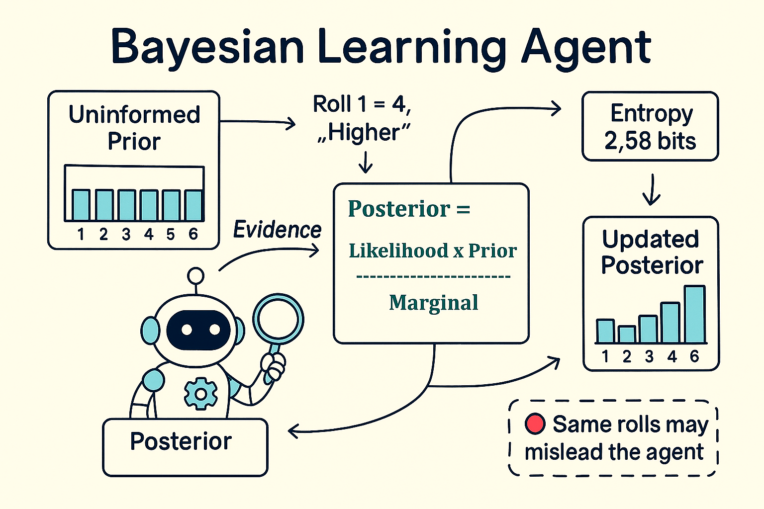
By creating this agent, we can learn the detail of the equation:
Posterior = (Likelihood × Prior) / Marginal
It is a great equation as it can be related to how we interpret information around us. How we make decisions, how different people can look at the same data and have different opinions and beliefs.
Applying the equation to a game
Let’s define a game. One where you have to guess a number. That number comes from a dice throw which you have not seen. To help you guess the number, there are further dice throws, and you are told if that throw is higher, lower, or the same as the original throw. We’ll refer to the original throw as the Target and the subsequent throws as the Evidence.
As an example
| event | Player 1’s knowledge | Player 2’s knowledge - the evidence |
|---|---|---|
| Start | The Target (e.g. 3) | An uninformed prior (e.g. all possibilities are equal) |
| Roll 1 | 4 | Higher - updates probability distribution |
| Roll 2 | 1 | Lower - updates probability distribution |
And so on…
What Player 2 must do is review the evidence, specifically the likelihood that the evidence occurs given its prior understanding, and produce a new belief of what the number is, that is the posterior. It is important to remember that these are Probability Distributions, not singular probabilities. As this is a discrete probability distribution, we will be able to iterate over singular probabilities for each Target value (i.e. all the values on the die).
Let’s break down the components of the equation (and also bring in the marginal):
- The Posterior Probability: P(Target | Evidence)
This is what we’re trying to calculate - the updated belief about each possible target value after observing evidence. It is a Probability Distribution.
- The Likelihood: P(Evidence | Target)
This is the probability of observing the evidence if a particular target were true. We iterate over the Probability Distribution here and calculate the likelihood for each Target.
- The Prior: P(Target)
Our belief about each target value before seeing new evidence. Initially uniform (1/6 for each value), but gets updated with each round.
- The Marginal: P(Evidence)
The probability of observing this evidence across all possible targets. This ensures our posterior probabilities sum to 1.
Seeing the distributions
I think it helps to see the distributions, so here is an uninformed prior and two posteriors, one after Roll 1 and another after Roll 2.
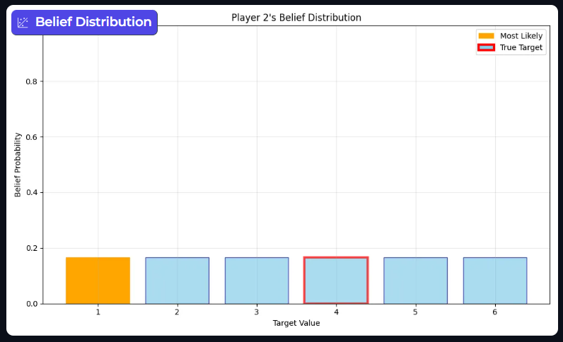 This bar graph displays Player 2’s belief distribution before the game starts, the belief probabilities are for target values 1 to 6, the prior is uninformed.
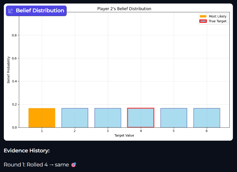 This bar graph displays Player 2’s belief distribution after a Roll. However the evidence provided is that Roll 1 is the same value as the Target value. As such, even though we performed the calculations, we have no evidence that changes our original prior.
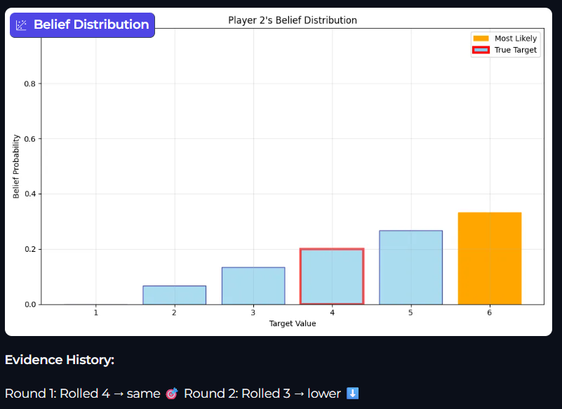 This bar graph displays Player 2’s belief distribution after another Roll. This time Player 2 receives the evidence that Roll 2 is higher the Target value. Calculating the posterior means that we get a new belief on what the Target value could be.
One thing to note, you may have used some Symbolic Logic here, and thought “of course 1 is no longer present, there is no Target below 1 so no rolls can be lower than that”. This is perfectly valid and, in effect what is occurring, however it is still completely by Bayes Theorem and ends up at the same result because the likelihood that we see Evidence higher with a Target of 1 is zero.
From Math to Code
Calculating the likelihood
The likelihood calculation is the heart of the Bayesian engine. For basic evidence (“higher”, “lower”, “same”), this is straightforward - :
class BayesianBeliefState:
    """Bayesian belief state for inferring target die value.

    Handles pure Bayesian inference without knowledge of actual values.
    """
...

    def update_beliefs(self, evidence: BeliefUpdate) -> None:
        """Update beliefs based on new evidence using Bayes' rule.

        Args:
            evidence: New evidence to incorporate
        """

        self.evidence_history.append(evidence)

        comparison_result = evidence.comparison_result

        # Calculate likelihood for each possible target value
		# Start with likelihoods of zero
        likelihoods = np.zeros(self.dice_sides)

		# The objective is to guess the number from the first throw of the die.
		# As such, the probability distribution is over the number of sides on the die.
        for target_idx in range(self.dice_sides):
            target_value = target_idx + 1

            # Calculate P(evidence.comparison_result | target_value)
            # This is the probability that ANY dice roll would produce this comparison result
            if comparison_result == "higher":
                # P(roll > target) = (dice_sides - target) / dice_sides
                likelihood = (self.dice_sides - target_value) / self.dice_sides
            elif comparison_result == "lower":
                # P(roll < target) = (target - 1) / dice_sides
                likelihood = (target_value - 1) / self.dice_sides
            else:  # comparison_result == "same"
                # P(roll = target) = 1 / dice_sides
                likelihood = 1 / self.dice_sides

            likelihoods[target_idx] = likelihood
This bit of code will produce an array of probabilities, an example for lower when using a 6-sided die is: [0, 1/6, 2/6, 3/6, 4/6, 5/6]
These probabilities are due to the number of dice rolls that satisfy the condition of being lower than the target
Target=1: P(roll < 1) = 0/6     (no rolls work)
Target=2: P(roll < 2) = 1/6     (roll=1 works)
Target=3: P(roll < 3) = 2/6     (roll=1,2 work)
Target=4: P(roll < 4) = 3/6     (roll=1,2,3 work)
Target=5: P(roll < 5) = 4/6     (roll=1,2,3,4 work)
Target=6: P(roll < 6) = 5/6     (roll=1,2,3,4,5 work)
One thing that is clear is that these probabilities do not add up to one. Bayes Theorem accommodates this by normalising the distribution, it divides the product of the prior and the likelihood (called the posterior_unnormalized in the code) by the marginal (i.e. the sum of the unnormalised posterior).
The Marginal: Updating the beliefs to a normalised posterior
The class starts with a uninformed prior; it sets the self.beliefs variable to a uninformed probability distribution where each is as likely as the other.
The self.beliefs value will then be updated with the normalised posterior after evidence has been processed. This is the importance of the marginal, it returns the posterior to a distribution that sums to 1.
class BayesianBeliefState:
    """Bayesian belief state for inferring target die value.

    Handles pure Bayesian inference without knowledge of actual values.
    """

    def __init__(self, dice_sides: int = 6):
        """Initialize belief state with uniform prior.

        Args:
            dice_sides: Number of sides on the dice
        """
        self.dice_sides = dice_sides
        # Uniform prior over all possible target values
        self.beliefs = np.ones(dice_sides) / dice_sides

...


    def update_beliefs(self, evidence: BeliefUpdate) -> None:

...

        # Calculate unnormalized posterior: prior * likelihood
        posterior_unnormalized = self.beliefs * likelihoods

        # Calculate marginal: P(evidence) = sum of (prior * likelihood) for all targets
        marginal = np.sum(posterior_unnormalized)

        # Apply Bayes' rule: posterior = (prior * likelihood) / marginal
        if marginal > 0:
            self.beliefs = posterior_unnormalized / marginal
        else:
            # If all likelihoods are 0 (shouldn't happen with valid evidence),
            # reset to uniform distribution
            self.beliefs = np.ones(self.dice_sides) / self.dice_sides
Information Theory and measuring Uncertainty
Something that is informative and has been previously touched on is the entropy of a probability distribution. That is, how much information is present.
Entropy is calculated by summing the probability distribution multiplied by its log (to base 2): H = -Σ p(x) log₂(p(x))
The result, measured in bits, will be between 0 and log₂(6) ≈ 2.58 bits for a 6-sided die:
- High entropy (≈2.58 bits): Maximum uncertainty, uniform beliefs
- Low entropy (≈0 bits): High certainty, concentrated beliefs
- Absolute certainty (0 bits): Complete certainty about the target
The code used to calculate this is like so:
    def get_entropy(self) -> float:
        """Calculate entropy of current belief distribution.

        Returns:
            Entropy in bits (higher = more uncertain)
        """
        # Avoid log(0) by filtering out zero probabilities
        non_zero_beliefs = self.beliefs[self.beliefs > 0]
        if len(non_zero_beliefs) == 0:
            return 0.0
        return -np.sum(non_zero_beliefs * np.log2(non_zero_beliefs))
The benefit of entropy is that you have one number that gives you an indication of the (un)certainty in a probability distribution. It does not equate to being correct though.
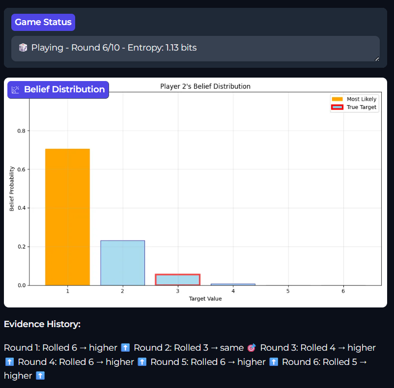
If you play the basic game on my Hugging Face space you can see that often, when the target is 3 or 4, sometimes 2 or 5, the agent will believe something that is incorrect. This happens more so when there are a series of throws that all result in the same number. For example, a series of 1s will make the agent believe that 6 is the most likely number, even if the target is 2. Over time the law of large numbers will balance things out, however in 10 rolls you can get mislead.
Extending the available evidence
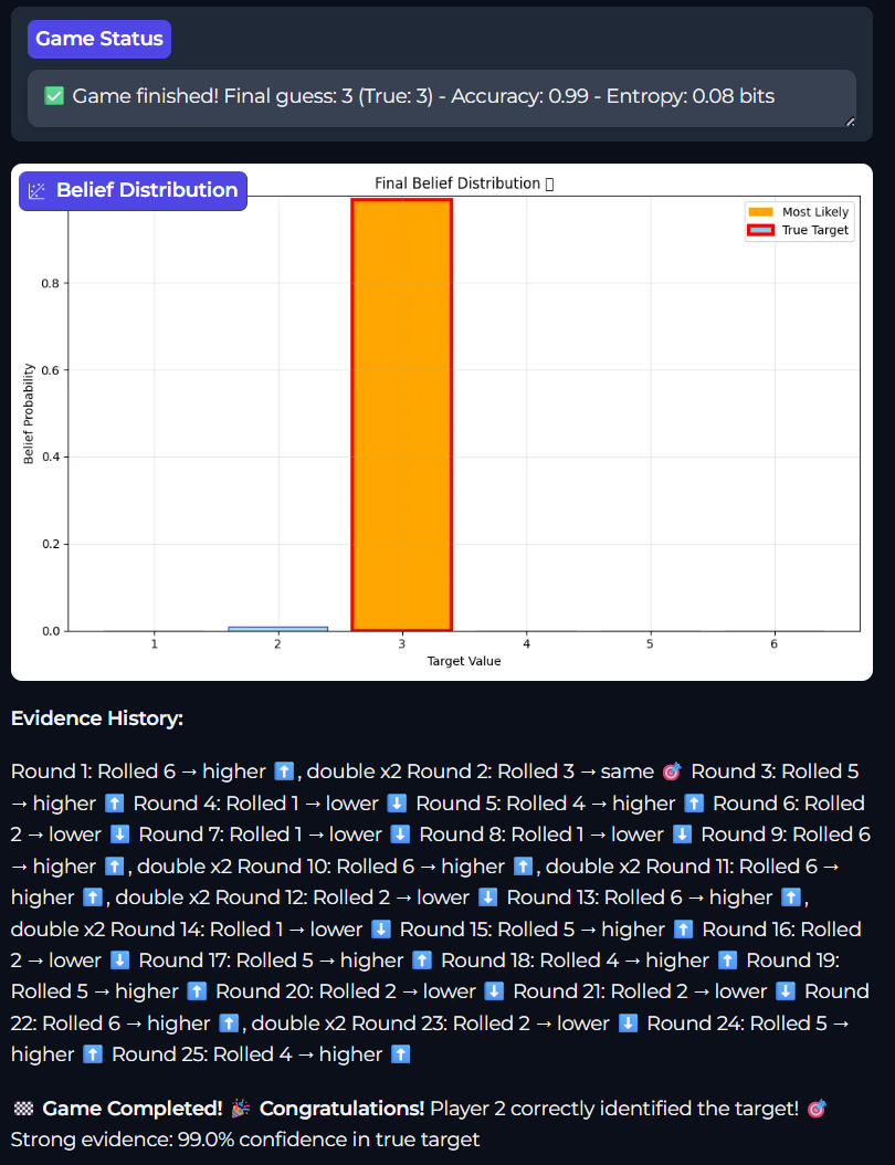
We are talking about the accuracy here, and one way to increase the accuracy of the belief is to get more evidence. As such there is an extended version of the game (available on the link above) that will also tell you if the number rolled is half or double of the target.
To do this the Belief code calculates the joint likelihood when two pieces of evidence are available. The update_beliefs method is updated to call the _calculate_joint_likelihood method:
    def update_beliefs(self, evidence: BeliefUpdate) -> None:

...

        # Calculate likelihood for each possible target value
        likelihoods = np.zeros(self.dice_sides)

        for target_idx in range(self.dice_sides):
            target_value = target_idx + 1

            # Calculate P(comparison_results | target_value)
            # This is the joint probability that a dice roll would produce ALL these evidence types
            likelihood = self._calculate_joint_likelihood(
                comparison_results, target_value
            )
            likelihoods[target_idx] = likelihood
	def _calculate_joint_likelihood(
        self, comparison_results: list[str], target_value: int
    ) -> float:
        """Calculate P(comparison_results | target_value) for multiple evidence types.

        Args:
            comparison_results: List of evidence results (e.g., ["lower", "half"])
            target_value: Target value to calculate likelihood for

        Returns:
            Joint probability of observing all evidence types given the target
        """
        # For multiple evidence types from a single roll, we need to find
        # the probability that a single dice roll satisfies ALL conditions

        # Count dice rolls that satisfy all evidence conditions
        satisfying_rolls = 0

        for dice_roll in range(1, self.dice_sides + 1):
            satisfies_all = True

            for evidence in comparison_results:
                if (
                    (evidence == "higher" and not (dice_roll > target_value))
                    or (evidence == "lower" and not (dice_roll < target_value))
                    or (evidence == "same" and dice_roll != target_value)
                    or (
                        evidence == "half"
                        and not (
                            target_value % 2 == 0 and dice_roll == target_value // 2
                        )
                    )
                    or (
                        evidence == "double"
                        and not (
                            dice_roll == target_value * 2
                            and dice_roll <= self.dice_sides
                        )
                    )
                ):
                    satisfies_all = False
                    break

            if satisfies_all:
                satisfying_rolls += 1

        return satisfying_rolls / self.dice_sides
This will rule out some targets - for example if the Player 1 (the environment) returns “lower” and “half” the Likelihood distribution is [0, 1/6, 0, 1/6, 0, 1/6].
Target=1: 0/6     (no rolls work)
Target=2: Must be roll=1 (half of 2), and 1 < 2 ✓ → 1/6
Target=3: 0/6     (no rolls work)
Target=4: Must be roll=2 (half of 4), and 2 < 4 ✓ → 1/6
Target=5: 0/6     (no rolls work)
Target=6: Must be roll=3 (half of 6), and 3 < 6 ✓ → 1/6
This extra evidence will increase the certainty in distribution as well as the accuracy. As we see here the entropy can drop to 0.08.
A note on evidence design
By adding half and double we enable the agent to be more accurate, however this will not identify all targets. specifically, with a six-sided die, 5 will not be highlighted as it has no half nor double that can occur. There will be similar numbers for dice of other sizes. Intuitively there should be a way to calculate which targets are excluded.
A further action of the game could be to calculate the probability that these unidentifiable numbers are the Target. This could be built into the calculation based on the number of rolls. This deserves further thought, particularly in relation to Markov Chains. In this implementation the Markov Property is present - each belief update depends only on the current state, not the full evidence history.
However, tracking “absence of evidence” would require remembering what evidence types we’ve seen across all rounds, potentially violating this memoryless property.
Conclusion
Here we have a method of updating the agents beliefs based on new evidence. If we look back at the previous post, the example was birds flying, more specifically Penguins cannot fly. We can represent the probability distribution like this:
P(fly | bird_type = penguin) = 0.01
P(fly | bird_type = ostrich) = 0.01
P(fly | bird_type = dodo) = 0.01
P(fly | bird_type = other) = 0.99     // The generic "flying bird" category
If you are standing in your back garden and you don’t live in South Africa, the Antarctic or the Australian bush, then you will have a prior that is similar to this :
P(bird_type = penguin) = 0.001     // Rare
P(bird_type = ostrich) = 0.001     // Rare
P(bird_type = dodo) = 0.0          // Extinct
P(bird_type = other) = 0.998       // Most birds are "generic flying birds"
The agent will go through the process of having a starting belief: “I see a bird”
- 99.8% chance it’s a generic flying bird → 99% chance it flies
- 0.2% chance it’s a flightless species → 1% chance it flies
Overall: ~98.8% chance this unknown bird can fly
And if your feet are very cold, you can only see white countryside, then the probability the bird you are looking at cannot fly increases massively.
The code!!
All the code is available on this GitHub repo