[NN Series 5/n] Regularisation: reducing the complexity of a model without compromising accuracy

Regularisation is known to reduce overfitting when training a neural network. As with a lot of these techniques there is a rich background and many options available, so asking the question why and how opens up to a lot of information. Diving through the information, for me at least, it wasn’t clear why/how it did this until I reframed what it was doing.

In short, regularisation changes the sensitivity of the model to the training data. In fact, not only can the sensitivity be reduced, you can tune it. Making the model more or less sensitive to features in the training data.This is also known as Variance, and can be seen as the amount the model will change if you change the training data.

So, yes it does reduce overfitting; however what it’s really doing is reducing the impact of features in the model. This is an example graph where I got the “aha moment”. The first graph has regularisation turned off and the second has regularisation fully turned on (note that the alpha value is used to calibrate the regularisation and that there are many types).

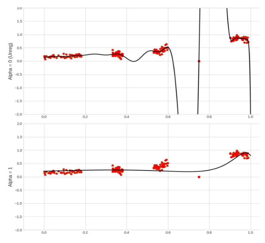
To put what I see into words, on this image there are two models, the first is complex and uses high order polynomials to include the outlining data point. This is not needed and will create erroneous predictions near the outlier (e.g. values like 0.7 or 0.9). By applying regularisation the model is smoothed out as the coefficients of high order polynomials are reduced, pushed towards zero.

Different Types of regularisation

For me this is an area that I need to look into deeper. Here I’ve listed three types of regularisation, I’ve not yet implemented them in a rigorous fashion so only can write about the principles.

L1 Regularisation

Add the weights into the loss calculation, effectively penalising the model for high weights.

Add the sum of the absolute values of the weights to the loss.

L2 Regularisation

AKA ridge regression or weight decay.

Add the sum of the squared values of the weights to the loss.

This exaggerates the impact of the high values compared to the low values.

A characteristic is that weights do not go to zero like in L1 Regularisation. Therefore you do not have a sparse neural network.

Drop out regularisation

AKA Make some neurons inactive.

The drop out rate is p and is the probability that, in each training step, a neuron is inactive.

The keep probability (1 -p) needs to be included in the inputs to accommodate missing neurons.

The alpha parameter

AKA how much attention to pay to the regularisation penalty.

Note:

• If the penalty is too strong: the model will underestimate the weights and underfit the problem.
• if the penalty is too weak: the model will be allowed to overfit the training data.

The value of alpha is between 0 (no penalty) and 1 (full penalty).

Other benefits

As well as the benefit of a simple less variant model, there are two other benefits that it has:

1. Training on less data than the number of features - allows us to interpolate models by using cross validation on a complementary dataset to direct the choice of regularisation parameters.
2. Sparsity - more efficient computationally, with memory, and energy use, it is more interpretable, and aligns to our understanding of biology.

Cross validation

AKA test as you go.

Whilst training with the val_loss

A recognised way to perform cross validation is to monitor the difference between the training loss and test loss whilst training.

The below image displays a negative training cycle, the diverging results show that the model is incorrectly fitted, in this case overfitting.

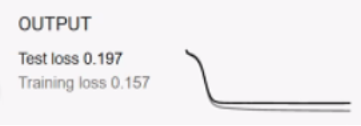
A graph with no convergence at the start would indicate the model being poorly fitted from the beginning and a change in bias (i.e. regularisation values) should be performed.

A cross validation example code for a MLP

from sklearn.model_selection import train_test_split

# Load the full MNIST dataset
(x_train, y_train), (x_test, y_test) = tf.keras.datasets.mnist.load_data()
# Resize the test dataset
x_test_resized = resize_mnist(x_test)
x_train_resized = resize_mnist(x_train)
# Reshape labels to match the expected format (m, 1)
y_train = y_train.reshape(-1, 1)
y_test = y_test.reshape(-1, 1)

# Step 1: Check original data shapes
print("x_train shape:", x_train.shape)
print("x_train_resized shape:", x_train_resized.shape)
print("y_train shape:", y_train.shape)

# Step 2: Split into train and validation sets (80-20 split here)
X_train, X_val, y_train, y_val = train_test_split(
    x_train_resized, y_train, test_size=0.2, random_state=42
)

# Step 3: Inspect the splits
print("X_train shape:", X_train.shape)
print("y_train shape:", y_train.shape)
print("X_val shape:", X_val.shape)
print("y_val shape:", y_val.shape)

# Ensure the test set is ready
print("x_test shape:", x_test.shape)
print("y_test shape:", y_test.shape)

A cross validation example in a q-learning agent

In the qlearning_maze_agent used when running an experiment

   def _run_single_experiment(self, config, save_path, experiment_id=None, iteration_count=None):
        """Execute single experiment with full metric collection"""
        env = MazeEnvironment(config)
        
        # Create directory and save maze visualization
        maze_path = Path(save_path)
        maze_path.mkdir(parents=True, exist_ok=True)
        self._save_maze_visualization(env, maze_path)
        
        # Save maze metadata
        maze_metadata = {
            'seed': env.seed,
            'grid': env.grid.tolist(),  # Convert numpy array to list for JSON
            'start': env.start,
            'end': env.end,
            'optimal_path': env.optimal_path,
            'optimal_path_length': env.optimal_path_length
        }
        with open(maze_path / 'maze_metadata.json', 'w') as f:
            json.dump(maze_metadata, f, indent=4)
            
        agent = QLearningAgent(env, config)
        control = AgentControl(env, agent, config)
        
        # Train and save training plot
        control.train(
            save_path=str(save_path),
            experiment_id=experiment_id,
            iteration_count=iteration_count
        )
        
        # Run consistency tests
        test_results = control.test_consistency(num_tests=10)

Conclusion

Regularisation is really powerful. It has practical benefits as well as secondary benefits. From a personal point of view this was really important for me to grasp. It was the feedback I got from my Neural Networks course submission. Interestingly it was a graph that meant the topic clicked and gave me the “aha moment”, normally it’s code… As such this post is largely therotical without example implementations and comparisons of regularisation. In a large part I do not have time. I do hope to revisit this and investigate the implementation of each of the types.

The question that I am left with is why would you not always use L2 Regularisation. From what I’ve read it is possible that it is always used. Probable even.

After that, I think a key thing to understand is the Drop Out Regularisation and the similarity to the Mixture of Experts architecture. However this is one for the future after Deep Learning and the Transformers architecture.